Graphs¶

Graph representation with adjacency matrix¶

Matrix representation of Graph

Arguments:¶

vertices (int): Number of total vertices in the graph
is_directed (Bool): Expects directed or not directed graph. Defaults to not directed graph.

Space Complexity:¶

Space complexity for graphs represented with adjacenecy matrix is $O(V^2)$ where $V$ is number of vertices. Use this method of representation only when your graph is dense. Number of edges $|E| ≥ V^2$ Else a lot of zeros will be placed inside the matrix which won’t be that efficient space wise. For sparse matrix use GraphDictionaryRepresented instead of GraphMatrixRepresented.

from AKDSFramework.structure.graph import GraphMatrixRepresented
import numpy as np

graph1 = GraphMatrixRepresented(vertices=10, is_directed=True)

# Now add few edges with random weights
while graph1.number_of_edges < 100:
    random_start = np.random.randint(low=0, high=graph1.vertices)
    random_end = np.random.randint(low=0, high=graph1.vertices)
    random_weight = np.random.randint(-7, 20)
    if random_weight != 0 and graph1.show_graph()[random_start][random_end] == 0:
        graph1.add_edge_between(start=random_start, end=random_end, weight=random_weight)
        graph1.add_edge_between(start=random_start, end=random_end, weight=random_weight)
    else:
        pass

      
    

Now showing edges and vertices and the matrix representation of the graph

print(f"Total number of edges: {graph1.number_of_edges}")  # or print(graph1.count_edges())
print(f"Total vertices: {graph1.vertices}")
print(graph1.show_graph())

Total number of edges: 100
Total vertices: 10
[[-6 -6 -4 -3  5 -7 -3 -6 13 -1]
 [ 4 -2 14 12  1  6 -5 -1 11 15]
 [12 12  9  9  8 -7  6 -2 13 19]
 [-5 -7 -1 19  1 15  2 17 13  9]
 [-4  6 -1  4 -5  1 -5 11 14 10]
 [ 7  2 19  7 10 -7 -7  9  8 14]
 [ 5 -4 -2  1  9  7  4  6 -1  8]
 [ 4  6 10  7  3  4 -3 15  6 14]
 [ 8 -4 12  3  2 10 -1 -1 -5 -1]
 [ 6 -3 -7 19  6 16 12  3 -3  1]]

Graph representation with adjacency lists¶

If you have a sparse graph use GraphDictionaryRepresented() for representing graphs. This takes $O(E + V)$ space. Running BFS DFS will be faster in this structure for sparse represented graphs, that’s why we implemented BFS DFS as a method in GraphDictionaryRepresented class.

Let’s create a graph¶

Let’s create a graph. To create graphs we need to create Vertex objects. We’ve made custom vertex objects because we need to store the neighbours and keep track of those guys.

from AKDSFramework.structure.graph import Vertex
from AKDSFramework.structure.graph import GraphDictionaryRepresented

g = GraphDictionaryRepresented()

Now let’s register few vertices:

for i in range(1, 8):
    g.register_vertex(Vertex(f'{i}'))

print(f"Now we have {g.number_of_vertices} number of vertices")

Now we have 7 number of vertices

Using raw_dict you can see all the vertices and their neighbors

print("Here is the dictionary containing all the vertices and it's neighbor")
g.raw_dict()

Here is the dictionary containing all the vertices and it's neighbor

{
    '1': <AKDSFramework.Vertex> object 1 with neighbors: [],
    '2': <AKDSFramework.Vertex> object 2 with neighbors: [],
    '3': <AKDSFramework.Vertex> object 3 with neighbors: [],
    '4': <AKDSFramework.Vertex> object 4 with neighbors: [],
    '5': <AKDSFramework.Vertex> object 5 with neighbors: [],
    '6': <AKDSFramework.Vertex> object 6 with neighbors: [],
    '7': <AKDSFramework.Vertex> object 7 with neighbors: []
}

As we’ve not registerd neighbor’s and edges with the vertex all the neighbors are showing blank. Let’s now add a few edges.

edges = ['15', '14', '12', '27', '26', '23']
for edge in edges:
    g.register_edge(edge[:1], edge[1:], directed=False)

Now let’s have a look at the graph

g.prettyprint()

1 -> [('2', 1), ('4', 1), ('5', 1)]

2 -> [('1', 1), ('3', 1), ('6', 1), ('7', 1)]

3 -> [('2', 1)]

4 -> [('1', 1)]

5 -> [('1', 1)]

6 -> [('2', 1)]

7 -> [('2', 1)]

And the dictionary would look like

g.raw_dict()

{
    '1': <AKDSFramework.Vertex> object 1 with neighbors: [('2', 1), ('4', 1), ('5', 1)],
    '2': <AKDSFramework.Vertex> object 2 with neighbors: [('1', 1), ('3', 1), ('6', 1), ('7',
1)],
    '3': <AKDSFramework.Vertex> object 3 with neighbors: [('2', 1)],
    '4': <AKDSFramework.Vertex> object 4 with neighbors: [('1', 1)],
    '5': <AKDSFramework.Vertex> object 5 with neighbors: [('1', 1)],
    '6': <AKDSFramework.Vertex> object 6 with neighbors: [('2', 1)],
    '7': <AKDSFramework.Vertex> object 7 with neighbors: [('2', 1)]
}

That’s our graph.

BFS & DFS¶

Let’s run BFS and DFS algo on top of the graph to see results. We’ll start from vertex number ‘1’

print(g.BFS('1'))
print(g.DFS('1'))

['1', '2', '4', '5', '3', '6', '7']
['1', '2', '3', '6', '7', '4', '5']

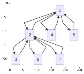
Visualize the graph¶

You can also see how your graph looks. Either in a TD (Top down approach) or a LR(Left right view).

from AKDSFramework.structure.graph import draw_graph
draw_graph(g, "TD")

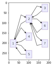
Left to right view of the same graph.

draw_graph(g, "LR")

AKDSFramework Documentation